11/01/20
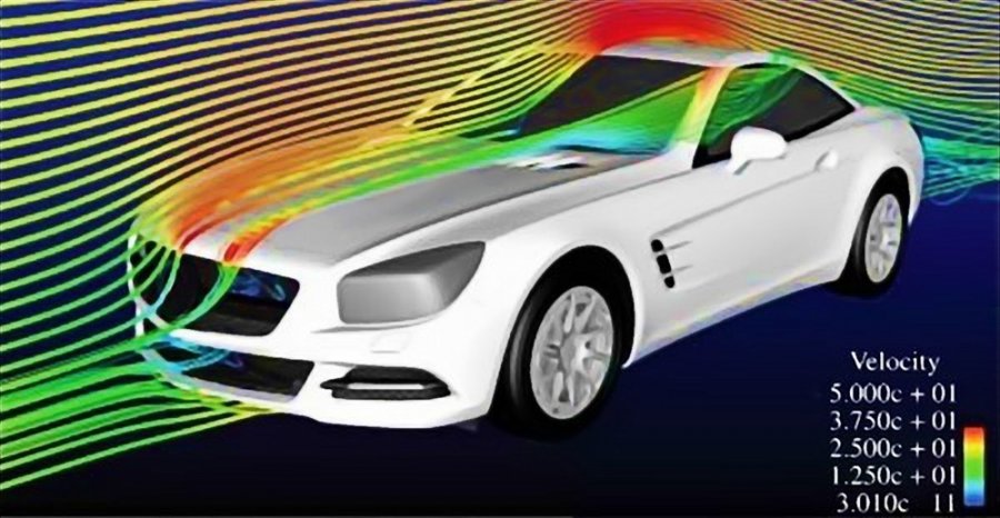
Aerodynamic drag is a force which resists vehicle motion and its magnitude is function of the speed. It depends on vehicle shape and size while its impact is greatest at higher speeds. While designing a purely urban vehicle its influence can be omitted or simplified to some degree but for more universal and common vehicles such as average class passenger car it cannot be disregarded. The article briefly describes the aerodynamic drag and methods of its estimation which can be used while designing or testing a vehicle. The presented statistical aerodynamic drag coefficients are helpful while in first stages of the design process while the described coast-down method is especially useful if the measurements can be done on a vehicle.
Drag force \(F_D\) in air as well as in any other fluid can be expressed by the equation
\[ {F_D} = \frac{1}{2}\rho \left( {V - {V_{wind}}} \right){\;^2}{C_D}A\]
A is total frontal area of the vehicle – cross section in plane normal to the direction of motion. In passenger cars it is in range 79%-84% of area calculated from width and height of the car. The area can be also estimated for such cars in mass range \(m∈(800,2000) kg\) with the formula
\[ A = 1.6 + 5.6 \cdot {10^{ - 4}}\left( {m - 765} \right)\]
Which for cars of \(m = 1500\;kg\) would give estimated frontal area of \(A \approx 2\;{m^2}\).
Table 1. Estimated frontal area for passenger vehicles.
| \(m [kg]\) | 800 | 1000 | 1200 | 1500 | 1400 | 1600 | 1800 |
| \(A [m^2]\) | 1.6196 | 1.7316 | 1.8436 | 2.0116 | 1.9556 | 2.0676 | 2.1796 |
The aero dynamical drag can be greatly influenced by atmospheric conditions and for that reason measurements and calculations should be done for certain parameters. The most commonly used are temperature 15\(^\circ\)C and pressure 1013.2 hPa which are equivalent to mass density of air \(\rho = 1.225\;kg/{m^2}\). The drag coefficient \({C_D}\) depends on shape of the vehicle and can by approximately determined by the coast-down test in which vehicle is slow down by the aero dynamical drag and rolling resistances from known initial speed (\({V_0})\) to final speed \(\left( {{V_f}} \right)\). The wind speed \({V_{wind}}\) is assumed to be zero. The value of \({C_D}\) for modern passenger cars is about \(0.2 - 0.3\).

The coast down test can be done using GPS data logging software to store vehicle speed and time of each measurement. To avoid error due to road slope and wind the test should be performed in both directions of the track possibly few times and results averaged. Clutch of the vehicle (if it has one) should be disengaged to stop transfer of power from powertrain moment of inertia.
Such test should be precise enough to accurately model the vehicle. It should be noted that the method takes in account other significant variable – rolling friction and thus all other forces are attributed to that parameter. This approach may limit accuracy, but is necessary as in practice both forces caused by the rolling friction and air drag are much greater than any other. The method is described in details as it is simple and useful.
By integrating both sides formula derived from aerodynamic drag summed with rolling resistance force \({F_D} + {F_r}\) expression
\[ dt = - \frac{1}{{\frac{{\rho A{C_D}V\left( t \right)}}{{2m}} + \frac{{{F_r}}}{m}}}dV\left( t \right)\]
the solution is obtained for initial speed \({V_0}\) and instantaneous speed \(V\left( t \right)\)
\[ t = \sqrt {\frac{{2{m^2}}}{{\rho A{C_D}{F_r}}}} \;{\left[ {{\rm{atan}}\left( {{V_0}\sqrt {\frac{{\rho A{C_D}}}{{2{F_r}}}} } \right) - {\rm{atan}}\left( {V\left( t \right)\sqrt {\frac{{\rho A{C_D}}}{{2{F_r}}}} } \right)} \right]^\;}\]
next substituting \(\beta = {V_0}\sqrt {\frac{{\rho A{C_D}}}{{2{F_r}}}}\) yields family of curves \({V_{ul}}\left( {{t_{ul}}} \right) = \frac{{V\left( t \right)}}{{{V_0}}}\left( {\frac{t}{T}} \right)\) with non-dimensional units scaled by initial speed and final time \(T\)
\[ \frac{{V\left( t \right)}}{{{V_0}}} = \frac{1}{\beta }\tan \left( {\left( {1 - \frac{t}{T}} \right)atan\left( \beta \right)} \right)\;\]
This formula can be used to find \(\beta\) of curve closes to the collected measurements (also nondimensionalised in the same way). After \(\beta\) is known the aerodynamic drag coefficient \({C_D}\;\)and rolling resistance force \({F_r}\) can be calculated
\[ {C_D} = \frac{{2m\beta {\bf{atan}}\left( \beta \right)}}{{{V_0}T\rho A}}\]
\[ {F_r} = \frac{{{V_0}m{\bf{atan}}\left( \beta \right)}}{{\beta T}}\]
Described process was done with Matlab® script using least square approximation and plotting closest curves for visualization.
Additionally influence of \(\beta\) on rolling resistance and air drag coefficient was plotted. It can be concluded that \(\beta\) has biggest influence on concavity of the curve (non-linear component corresponding to aerodynamic drag) and friction force on is mainly affected by the time T.
With all constants known the effect of air drag can be simulated numerically in Simulink®. For fully working model sign of the force has to be corrected to always correspond direction of movement or wind direction (as squaring removes the sign). It was done so using simple switch comparing to net speed to zero (additionally some kind of hysteresis block may be necessary if zero-crossing error would occur).

Aerodynamically drag creates also down-force on axles \({F_{z1}},\;{F_{z2}}\) improving handling and reducing slip. Race cars exhibit especially high down-force due to low suspension, rear wing and skirts incorporated in the design. During overtaking rapid changes in down-force (caused by drafting effect) along with high motor torque can cause high wheel slip and loss of handling.
